

- Build
- Mandelbrot overview
- The code and image
- Data.Complex
- Magnitude
- Instability
- Pixel mapping
- The magical math
- Drawing the image
- Adding colors
We’ve used a package written by Cies Breijs that we found on GitHub to generate the header art for the Validation course pages. haskell-fractal on GitHub. We liked the image this package generates, and the author included some LaTeX to generate a PDF version of the art. In theory, we like the ability to print this out and hang it over our desks. We haven’t actually done that, yet, but we might!
Build
The project structure here is simple, and we didn’t feel the need to change it. But it can be tricky to build due to foreign dependencies; for us, the build instructions in the README did not work as stated. We added a stack.yaml so it can be built with Stack now, for those who want to do that. Our fork of haskell-fractal.
Once we could build it, we found that it took a long time to generate the image. It makes a big image with lots of detail, although it took much less time when using the width and height values that we needed for our image. Just bear in mind that creating the image at the original size setting takes a little bit of time.
Mandelbrot overview
The original code, as we’ll explain in depth soon, produces a beautiful image, but it’s only grayscale and we wanted color. Initially, we were going to write a short post here about the changes that we made to generate a color image. However, as with a typical fractal program, color generation is intimately tied up with the image generation and fractal math itself. So we’re going to go ahead and analyze this code and talk about how fractals like the Mandelbrot set work. We’re assuming that you have at least seen images of the Mandelbrot set, and other fractal sets, and have some idea of their features. As we work through the code, we’ll get into more mathematical detail, but we want to start with a high-level overview of how programs like this work. If some of this is confusing or you don’t know some of the jargon, we encourage you to keep reading, because it will be explained in more detail and with concrete examples below.
Programs that generate images of the Mandelbrot or Julia sets have at their core a fairly simple equation involving complex numbers. We can write the function in Haskell like this, where c and z are complex numbers:
f c z = z^2 + cWhile the function is simple, what we care about is what happens under iteration; we need to keep calling f on the result of the previous calculation. Essentially, there are two patterns: for some complex numbers, the values of z under iteration remain stable within a certain bounded size, while for other points in the complex plane the iterates are not stable and will diverge – quickly or slowly – toward infinity. When we say “diverge toward infinity”, we mean that the magnitude of the z values will grow larger, although it might not be a steady monotonic growth. We’ll explain complex numbers and magnitude more below. For the Mandelbrot set, the initial value of z is always 0 and and we vary the value of c; for Julia sets, we fix the value of c and vary the values of z.
We generate an image of the Mandelbrot set by assigning a complex number, c, to each pixel and seeing what the behavior is at that pixel. If it’s stable and does not ever diverge toward infinity, we paint that pixel one color; the Mandelbrot set is the set of those values c where the behavior of 0 under iteration is stable. If z is unstable and will eventually, under some number of iterations, head toward infinity, we paint that pixel another color. If we want to, we can use more than two colors by painting pixels depending on how fast they head toward infinity or how wildly unstable the orbits of the iterates are. This is often accomplished by using the number of iterations on a given pixel as one of the inputs to the function that assigns an RGB (or similar) value to that pixel.
While we’re going to get into this in more detail below, let’s look at some concrete examples of what this means. For the Mandelbrot set, we want to fix the start value of z for every c at 0 and see what happens under iteration. For these examples, we’ll stick with real numbers because we think it’s fair to say that most of us have a harder time mentally following along with arithmetic over complex numbers, if only because we typically have less experience with it. However, all real numbers are also complex numbers, with the imaginary component being 0i. So, let’s begin by choosing 1 as our c value – we need to make our Haskell function above recursive as well, since iteration is the point:
f c z = f c z'
  where z' = z^2 + c

c = 1
z = 0

f 1 0 = f 1 (0^2 + 1)
      = f 1 (1^2 + 1)
      = f 1 (2^2 + 1)
      = f 1 (5^2 + 1)
--    ... and so on
That will never terminate as written, but we can already see what we need to see: the values of z will just keep getting larger and larger. So, this value of c (or, more precisely, the complex number associated with this real number, which would be 1 + 0i) is not in the Mandelbrot set. Let’s try another one, shall we – how about (-1) this time?
f c z = f c z'
  where z' = z^2 + c

c = (-1)
z = 0

f (-1) 0 = f (-1) (0^2 + (-1))
         = f (-1) ((-1)^2 + (-1))
         = f (-1) (0^2 + (-1))
         = f (-1) ((-1)^2 + (-1))
--       ... and so on
The very picture of stability: the value of z just keeps bouncing back and forth between (-1) and 0. It will never diverge away from this orbit, no matter how many times we keep applying this function to the values of z. So, the complex number (-1 + 0i) is indeed in the Mandelbrot set.
To some extent, using only real numbers for examples has given us an unfair picture of what stability and instability mean with regard to this equation. When we looked at the equation for c = 1, the values of z grow ever larger but they do so monotonically – they only ever grow larger – so what exactly is unstable about this? It’s difficult to see without using some more complex examples, so we’ll do that when we talk about complex numbers, below.
Of course, we can’t apply the function infinitely many times to a given pixel, so in practice we choose a number of iterations and say, well, if z hasn’t grown really big after, say, 200 iterations, then it’s probably stable. On the other hand, if z ever attains a magnitude greater than 2, it will diverge toward infinity.
If we were intending to draw Julia sets instead, we’d fix the value of c and look for values of z that are stable under the same iteration – we wouldn’t start z at 0 every time. The Mandelbrot set is all the values of c where z = 0 is stable; the Julia sets are all the values of z that are stable for a given, fixed value of c.
One of the characteristics of the Mandelbrot set is that it demonstrates self-similarity across different scales, which is why we can zoom in on portions of the Mandelbrot set and find near-repeats of the shape of the Mandelbrot set itself. Using multiple colors that depend on the number of iterations we tried before you could tell it was heading toward infinity, as many of us know, highlights complex and repeating patterns along the borders between stable and unstable – we see degrees of instability; we see fractal complexity. Recursive equations that produce fractal complexity like these are the essence of chaos theory, because tiny changes in the value of c can produce large variations in behavior and it’s almost impossible to predict what they’ll be.
The code and image
OK, let’s start to make this more concrete. This is the code, as written, that we’ll be stepping through:
import Codec.Picture  (generateImage, writePng)
import Data.Word      (Word8)
import Data.Complex   (Complex(..), magnitude)

aspectRatio :: Double
aspectRatio = sqrt 2  -- nice cut for ISO216 paper size

x0, y0, x1, y1 :: Double
(x0, y0) = (-0.8228, -0.2087)
(x1, y1) = (-0.8075, y0 + (x1 - x0) * aspectRatio)

width, height :: Int
(width, height) = (10000, round . (* aspectRatio) . fromIntegral $ width)

maxIters :: Int
maxIters = 1200

fractal :: RealFloat a => Complex a -> Complex a -> Int -> (Complex a, Int)
fractal c z iter
    | iter >= maxIters = (1 :+ 1, 0)  -- invert values inside the holes
    | magnitude z > 2  = (z', iter)
    | otherwise        = fractal c z' (iter + 1)
  where
    z' = z * z + c

realize :: RealFloat a => (Complex a, Int) -> a
realize (z, iter) = (fromIntegral iter - log (log (magnitude z))) /
                     fromIntegral maxIters

render :: Int -> Int -> Word8
render xi yi = grayify . realize $ fractal (x :+ y) (0 :+ 0) 0
  where
    (x, y)           = (trans x0 x1 width xi, trans y0 y1 height yi)
    trans n0 n1 a ni = (n1 - n0) * fromIntegral ni / fromIntegral a + n0
    grayify f        = truncate . (* 255) . sharpen $ 1 - f
    sharpen v        = 1 - exp (-exp ((v - 0.92) / 0.031))

main :: IO ()
main = writePng "out.png" $ generateImage render width height
That code produces this image as output.
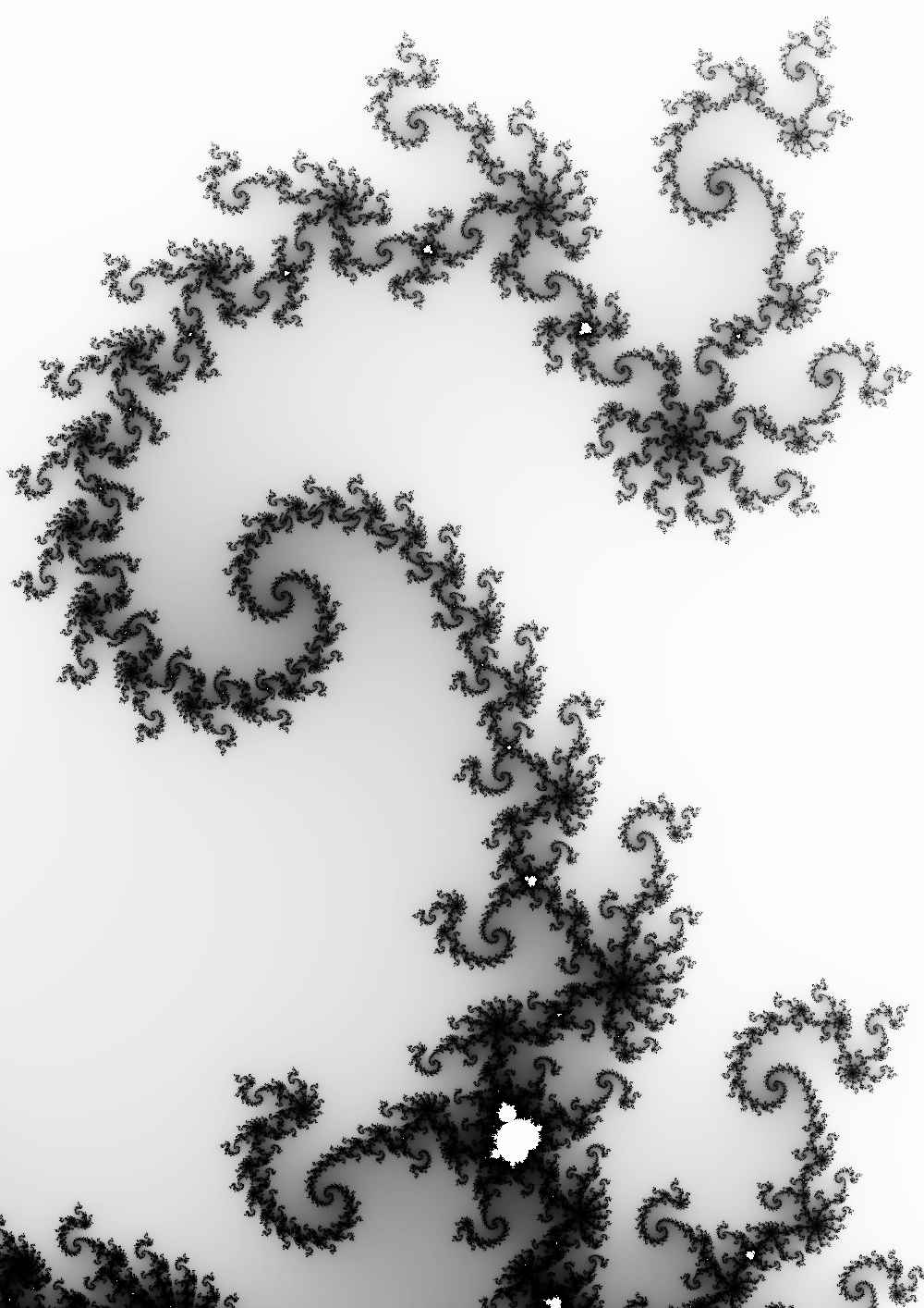
We’ll work through the code mostly top to bottom, explaining the math in more detail than we did above as we go along. We’ll also show the changes we made to make a color image. It’s worth immediately noticing that the function we referenced earlier on, f c z = z^2 + c, is in the fractal function in this program. We’ll examine it in greater detail below.